Delineamento Completamente Casualizado
Adilson dos anjos
Dados como exemplo
Carregar os dados
As variáveis precisam estar nessas classes
Resumo dos dados
##       trat         resp
##  t1     : 6   Min.   :115.0
##  t2     : 6   1st Qu.:307.5
##  t3     : 6   Median :377.5
##  t4     : 6   Mean   :353.5
##  t5     : 6   3rd Qu.:417.0
##  t6     : 6   Max.   :474.0
##  (Other):18
Média de cada tratamento
##       t1       t2       t3       t4       t5       t6       t7       t8
## 378.6667 431.5000 346.3333 293.6667 341.8333 406.0000 164.1667 403.8333
##       t9
## 415.6667
Variância dos tratamentos
##       t1       t2       t3       t4       t5       t6       t7       t8
## 1916.267  987.500 3117.867 3494.667 1513.767 1903.600 2173.367 1242.167
##       t9
## 1091.067
Tabela da ANOVA
Teste para saber se há diferença entre os tratamentos.
\[H_0: \mu_1 = \mu_2 = ... = \mu_i\] \[H_1: \mu_i \neq \mu_j\] #### Mesma coisa que:
\[H_0: \text{Diferença entre tratamentos não é significativa}\] \[H_0: \text{Diferença entre tratamentos é significativa}\]
##             Df Sum Sq Mean Sq F value   Pr(>F)
## trat         8 332918   41615   21.48 5.44e-13 ***
## Residuals   45  87201    1938
## ---
## Signif. codes: 0 '***' 0.001 '**' 0.01 '*' 0.05 '.' 0.1 ' ' 1## Analysis of Variance Table
##
## Response: resp
## Df Sum Sq Mean Sq F value Pr(>F)
## trat 8 332918 41615 21.475 5.445e-13 ***
## Residuals 45 87201 1938
## ---
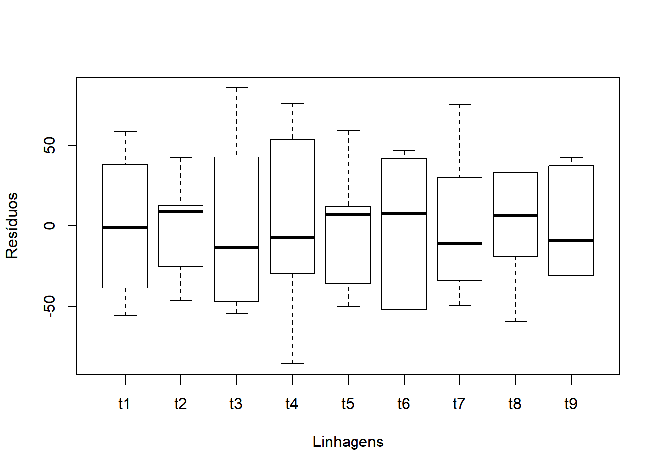
## Signif. codes: 0 '***' 0.001 '**' 0.01 '*' 0.05 '.' 0.1 ' ' 1Conferindo Homocedasticidade
\[H_0: \sigma^2_1 = \sigma^2_2 = ... = \sigma^2_i \] \[H_1: \sigma^2_i \neq \sigma^2_{i'} \text{ para pelo menos um } i \neq i'\]
Conferindo com bloxplot Tratamentos x Resíduos
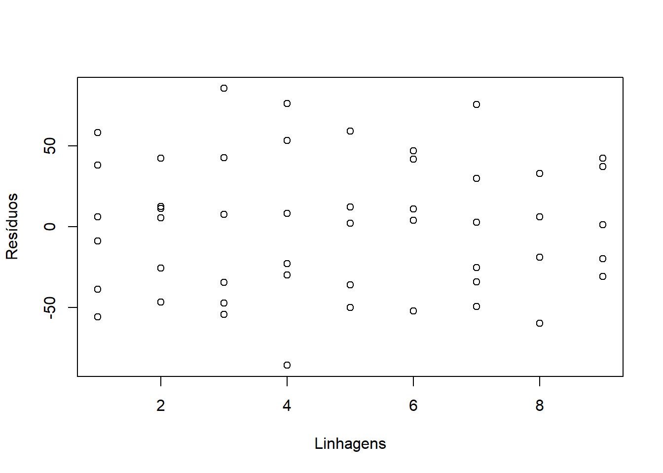
####Conferindo com Scatterplot Tratamentos x Resíduos
Conferindo com o teste Bartlett
##
##  Bartlett test of homogeneity of variances
##
## data:  ex01.av$res and ex01$trat
## Bartlett's K-squared = 3.6738, df = 8, p-value = 0.8853
Conferindo normalidade
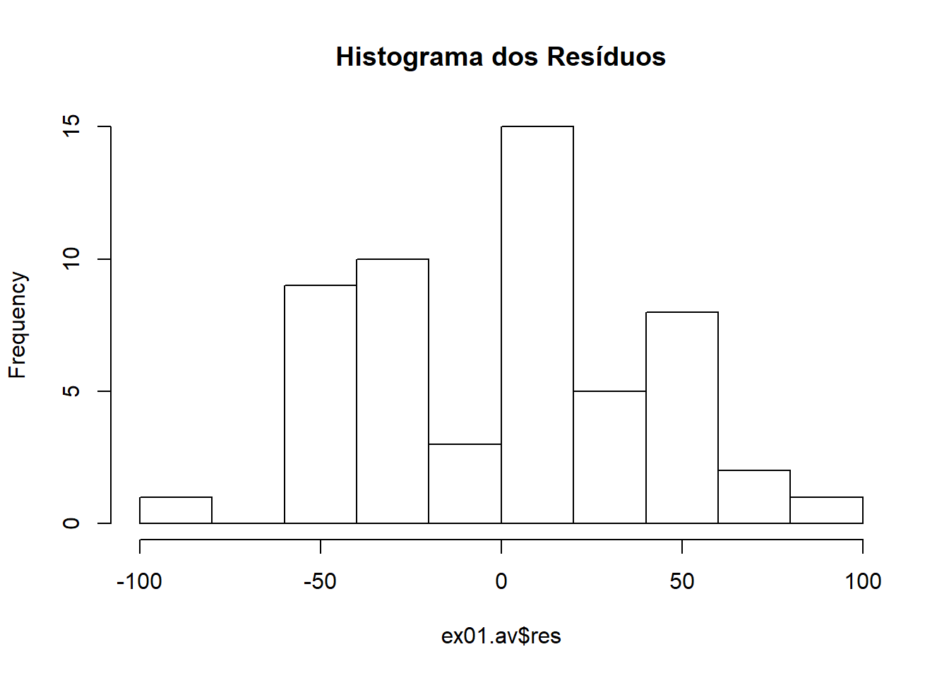
\[H_0: \text{erros possuem distribuição normal}\] \[H_1: \text{erros não possuem distribuição normal}\] #### Conferindo normalidade com histograma dos resíduos
Conferindo normalidade com gráfico de ramo e folhas
##
##   The decimal point is 1 digit(s) to the right of the |
##
##    -8 | 6
##    -6 | 0
##    -4 | 64220977
##    -2 | 96441106530
##    -0 | 99
##     0 | 123466668812222
##     2 | 03378
##     4 | 22337389
##     6 | 66
##     8 | 6
Conferindo normalidade com o gráfico normal de probabilidade dos resíduos
qqnorm(ex01.av$res,ylab="Resíduos", main=NULL)
qqline(ex01.av$res)
title("Grafico Normal de Probabilidade dos Resíduos")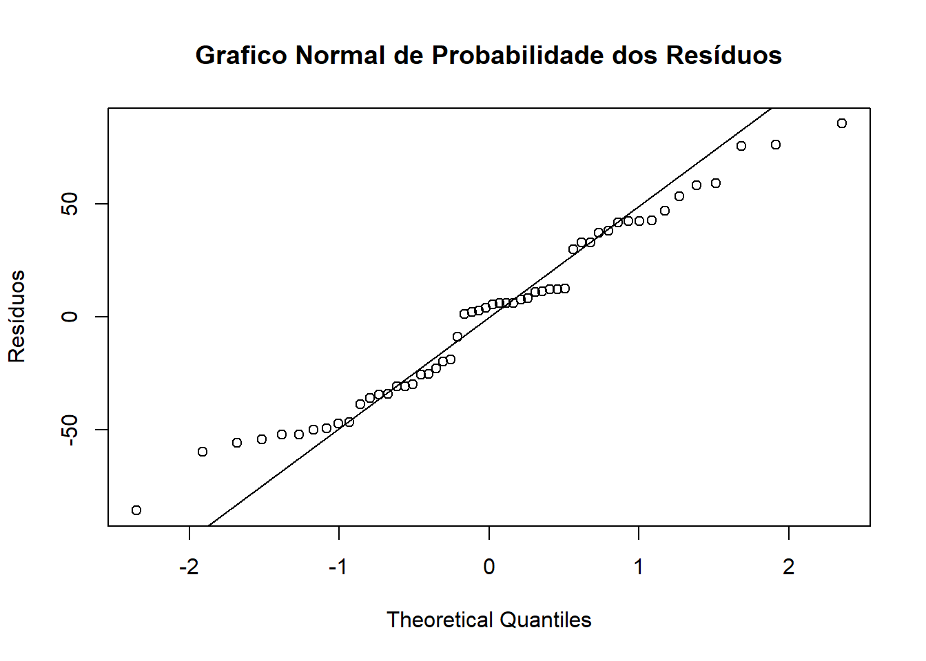
Conferindo normalidade com o teste Shapiro-Wilk
##
##  Shapiro-Wilk normality test
##
## data:  ex01.av$res
## W = 0.97159, p-value = 0.2263
Conferindo independência
Conferindo independência com o gráfico Scatterplot Valores ajustados x Resíduos
plot(ex01.av$fit, ex01.av$res, xlab="valores ajustados", ylab="resíduos")
title("resíduos vs Preditos")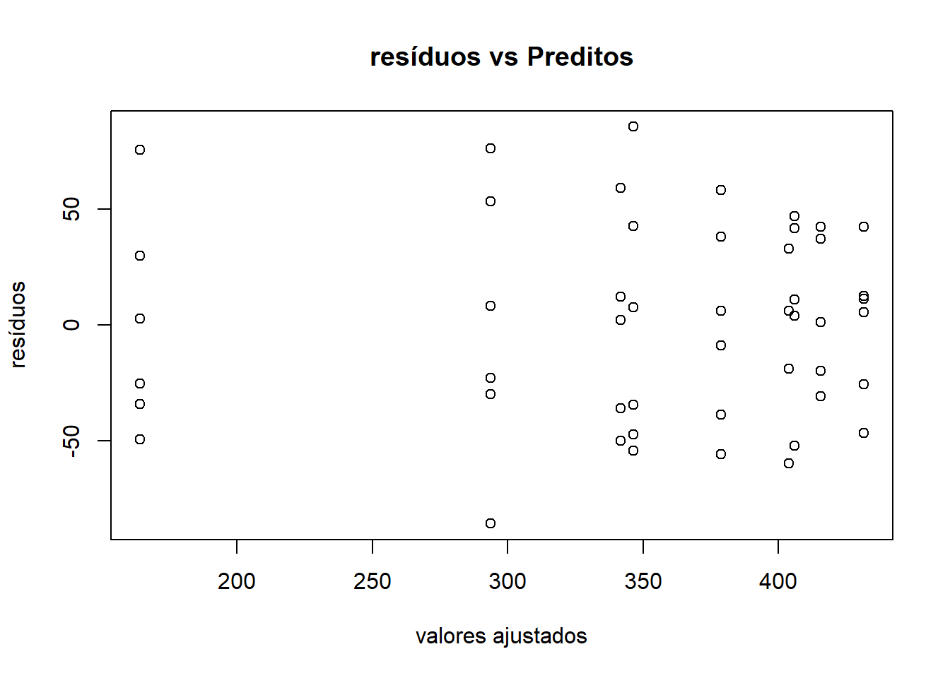
Conferindo independência com o gráfico Scatterplot Valores ajustados Ordenados x Resíduos
plot(ex01.av$fit, order(ex01.av$res), xlab="valores ajustados", ylab="resíduos")
title("resíduos vs Preditos")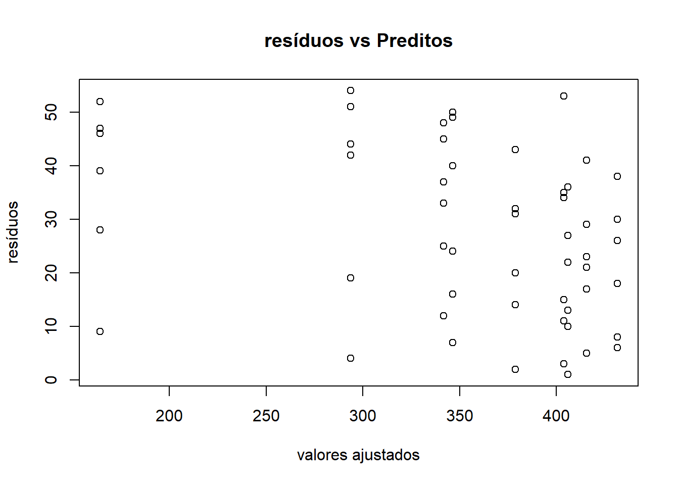
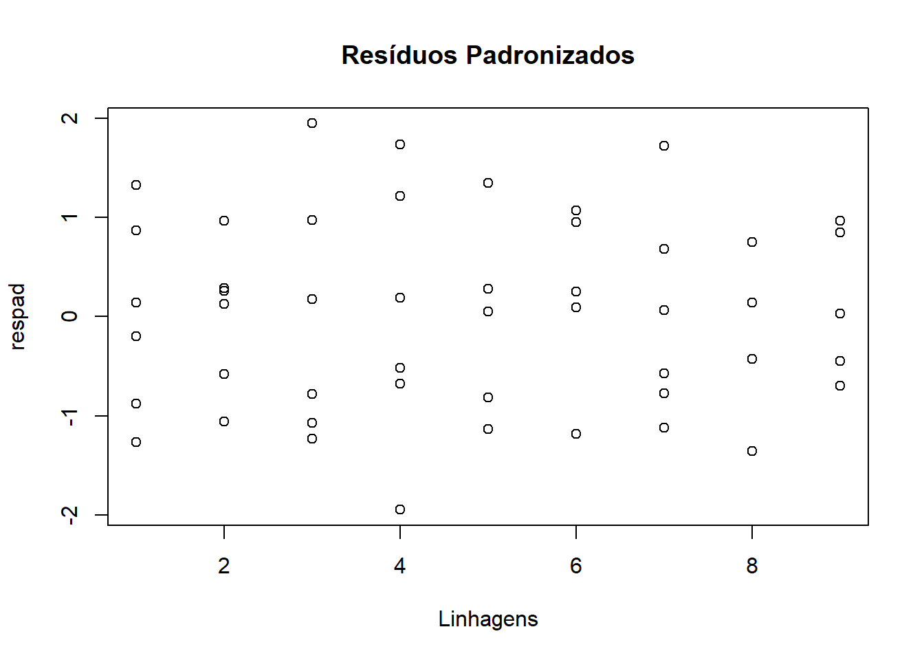
Verificação de Outliers
## [1] "Df" "Sum Sq" "Mean Sq" "F value" "Pr(>F)"s2 <- anova(ex01.av)$Mean[2] #### estimativa da variância
res <- ex01.av$res #### extraindo resíduos
respad <- (res/sqrt(s2)) #### resíduos padronizados
boxplot(respad)
title("Resíduos Padronizados" )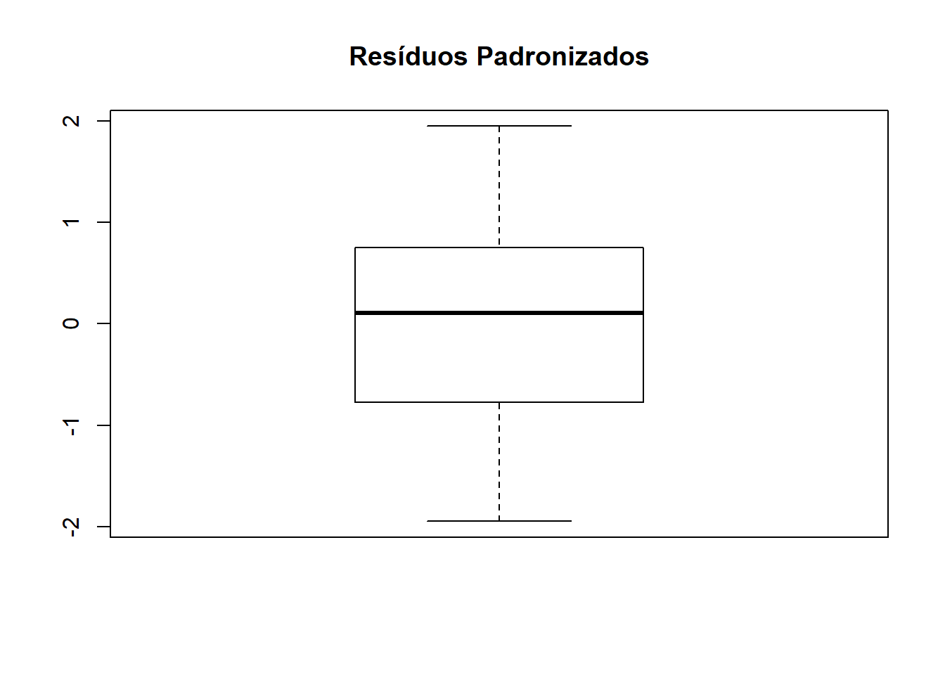
Teste Tukey
\[H_0: \mu_i = \mu_j\] \[H_1: \mu_i \neq \mu_j\] #### Mesma coisa que
\[H_0: \text{o constraste não é significativo}\] \[H_1: \text{o constraste é significativo}\]
Se 0 não estiver incluído no intervalo, rejeita-se a hipóte-se nula.
##   Tukey multiple comparisons of means
##     95% family-wise confidence level
##
## Fit: aov(formula = resp ~ trat, data = ex01)
##
## $trat
##              diff         lwr         upr     p adj
## t2-t1   52.833333  -29.947633  135.614299 0.4998060
## t3-t1  -32.333333 -115.114299   50.447633 0.9342210
## t4-t1  -85.000000 -167.780966   -2.219034 0.0401018
## t5-t1  -36.833333 -119.614299   45.947633 0.8721075
## t6-t1   27.333333  -55.447633  110.114299 0.9749062
## t7-t1 -214.500000 -297.280966 -131.719034 0.0000000
## t8-t1   25.166667  -57.614299  107.947633 0.9849417
## t9-t1   37.000000  -45.780966  119.780966 0.8693183
## t3-t2  -85.166667 -167.947633   -2.385701 0.0394343
## t4-t2 -137.833333 -220.614299  -55.052367 0.0000730
## t5-t2  -89.666667 -172.447633   -6.885701 0.0247945
## t6-t2  -25.500000 -108.280966   57.280966 0.9836416
## t7-t2 -267.333333 -350.114299 -184.552367 0.0000000
## t8-t2  -27.666667 -110.447633   55.114299 0.9730043
## t9-t2  -15.833333  -98.614299   66.947633 0.9993743
## t4-t3  -52.666667 -135.447633   30.114299 0.5040619
## t5-t3   -4.500000  -87.280966   78.280966 1.0000000
## t6-t3   59.666667  -23.114299  142.447633 0.3369467
## t7-t3 -182.166667 -264.947633  -99.385701 0.0000002
## t8-t3   57.500000  -25.280966  140.280966 0.3855262
## t9-t3   69.333333  -13.447633  152.114299 0.1671352
## t5-t4   48.166667  -34.614299  130.947633 0.6203900
## t6-t4  112.333333   29.552367  195.114299 0.0018566
## t7-t4 -129.500000 -212.280966  -46.719034 0.0002153
## t8-t4  110.166667   27.385701  192.947633 0.0024139
## t9-t4  122.000000   39.219034  204.780966 0.0005599
## t6-t5   64.166667  -18.614299  146.947633 0.2479215
## t7-t5 -177.666667 -260.447633  -94.885701 0.0000004
## t8-t5   62.000000  -20.780966  144.780966 0.2886707
## t9-t5   73.833333   -8.947633  156.614299 0.1146645
## t7-t6 -241.833333 -324.614299 -159.052367 0.0000000
## t8-t6   -2.166667  -84.947633   80.614299 1.0000000
## t9-t6    9.666667  -73.114299   92.447633 0.9999849
## t8-t7  239.666667  156.885701  322.447633 0.0000000
## t9-t7  251.500000  168.719034  334.280966 0.0000000
## t9-t8   11.833333  -70.947633   94.614299 0.9999286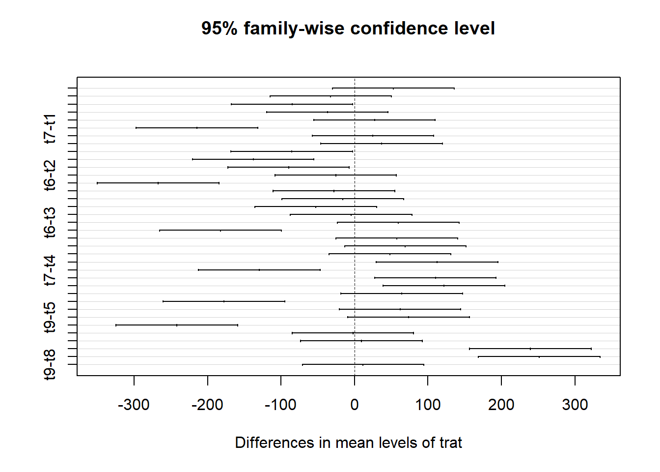
####Observando contrastes específicos de interesse
\[y_1 = 1/4 L_1 + 1/4 L_2 + 1/4 L_3 + 1/4 L_4 - 1/5 L_5 - 1/5 L_6 - 1/5 L_7 - 1/5 L_8 - 1/5 L_9\] \[y_2 = 1L_1 + 1L_2 - 1L_3 - 1L_4\] \[y_3 = 1L_1 - 1L_2\] \[y_4 = 1L_3 - 1L_4\] \[y_5 = 1L_5 + 1L_6 + 1L_7 + 1L_8 - 4L_9\] \[y_6 = 1L_5 + 1L_6 - 1L_7 - 1L_8\] \[y_7 = 1L_5 - 1 L_6\] \[y_8 = 1L_7 - 1L_8\]
Colocar os contrastes numa matriz
cont.ex01<-matrix(c(.25,.25,.25,.25,-.2,-.2,-.2,-.2,-.2,1,1,-1,-1,0,0,0,0,0,1,-1,0,0,0,0,0,0,0,0,0,1,-1,0,0,0,0,0,0,0,0,0,1,1,1,1,-4,0,0,0,0,1,1,-1,-1,0,0,0,0,0,1,-1,0,0,0,0,0,0,0,0,0,1,-1,0),nrow=9,ncol=8,byrow=F)
cont.ex01
## [,1] [,2] [,3] [,4] [,5] [,6] [,7] [,8]
## [1,] 0.25 1 1 0 0 0 0 0
## [2,] 0.25 1 -1 0 0 0 0 0
## [3,] 0.25 -1 0 1 0 0 0 0
## [4,] 0.25 -1 0 -1 0 0 0 0
## [5,] -0.20 0 0 0 1 1 1 0
## [6,] -0.20 0 0 0 1 1 -1 0
## [7,] -0.20 0 0 0 1 -1 0 1
## [8,] -0.20 0 0 0 1 -1 0 -1
## [9,] -0.20 0 0 0 -4 0 0 0Analisar os contrastes
Análise de Variância
Contrastes significativos
##             Df Sum Sq Mean Sq F value   Pr(>F)
## trat         8 332918   41615  21.475 5.44e-13 ***
##   trat: y1   1   3517    3517   1.815   0.1846
##   trat: y2   1  43435   43435  22.415 2.22e-05 ***
##   trat: y3   1   8374    8374   4.321   0.0434 *
##   trat: y4   1   8321    8321   4.294   0.0440 *
##   trat: y5   1  36088   36088  18.623 8.62e-05 ***
##   trat: y6   1  48510   48510  25.033 9.10e-06 ***
##   trat: y7   1  12352   12352   6.374   0.0152 *
##   trat: y8   1 172320  172320  88.925 3.16e-12 ***
## Residuals   45  87201    1938
## ---
## Signif. codes:  0 '***' 0.001 '**' 0.01 '*' 0.05 '.' 0.1 ' ' 1