Número de consultas ao médico

Modelos para dados com excesso de zeros

require("faraway")
require("gamlss")
help(dvisits)

Vamos modelar o número de visitas ao médico nas duas últimas semanas (doctorco) em função de algumas das covariáveis disponíveis na base

dvisits <- dvisits[sample(1:nrow(dvisits)),]

Apenas ordenando as linhas da base de forma aleatória (estavam dispostas de forma sistemática).

dvisits$sex <- as.factor(dvisits$sex)
levels(dvisits$sex) <- c('Masculino', 'Feminino')
dvisits$levyplus <- factor(dvisits$levyplus)
levels(dvisits$levyplus) <- c('Publico', 'Particular')
dvisits$chcond1 <- factor(dvisits$chcond1)
levels(dvisits$chcond1) <- c('Nao cronico', 'Cronico')

Convertendo algumas das variáveis para fator e renomeando os níveis.

tabela <- table(dvisits$doctorco)
barplot(tabela)

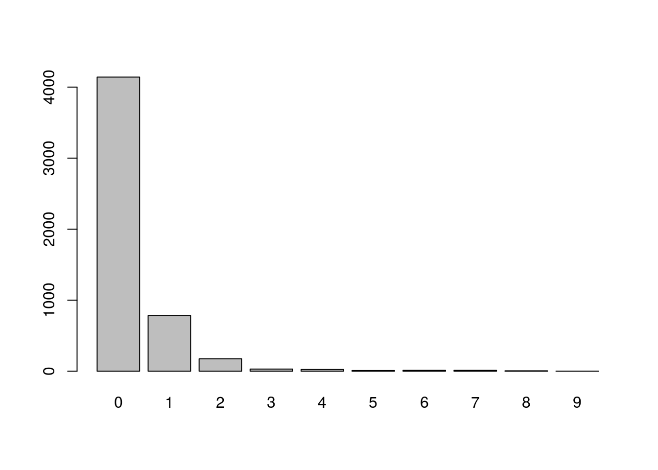
O gráfico de barras evidencia uma grande freqência de indivíduos com zero consultas.

Todos os ajustes na sequência foram realizados usando a biblioteca gamlss (mesmo aqueles que poderiam ser feitos usando a função glm, para fins de padronização).

Vamos avaliar os ajustes de seis modelos distintos:

Modelo 1: Poisson

(sem inflação de zeros)

modelo1 <- gamlss(doctorco ~ sex + age + agesq 
                  + income + levyplus + illness + actdays + chcond1 + hospadmi 
                  + medicine, family = PO, data = dvisits)

## GAMLSS-RS iteration 1: Global Deviance = 6628.372 
## GAMLSS-RS iteration 2: Global Deviance = 6628.372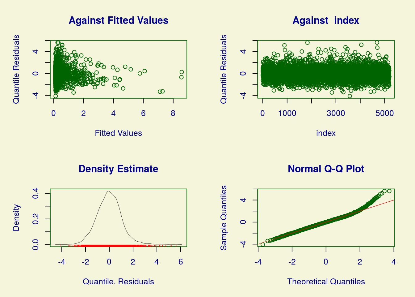

plot(modelo1)

## ******************************************************************
##   Summary of the Randomised Quantile Residuals
##                            mean   =  -0.004735209 
##                        variance   =  1.063899 
##                coef. of skewness  =  0.3654912 
##                coef. of kurtosis  =  4.383663 
## Filliben correlation coefficient  =  0.9935205 
## ******************************************************************

A biblioteca gamlss tem como padrão os resíduos quantílicos aleatorizados. O qqplot indica a não normalidade dos resíduos e, consequentemente, o desajuste do modelo.

Modelo 2: Binomial negativa

(sem inflação de zeros)

modelo2 <- gamlss(doctorco ~ sex + age + agesq + income + levyplus + illness + 
                      actdays + chcond1 + hospadmi + medicine, family = NBI, 
                  data = dvisits)

## GAMLSS-RS iteration 1: Global Deviance = 6370.117 
## GAMLSS-RS iteration 2: Global Deviance = 6357.454 
## GAMLSS-RS iteration 3: Global Deviance = 6357.372 
## GAMLSS-RS iteration 4: Global Deviance = 6357.372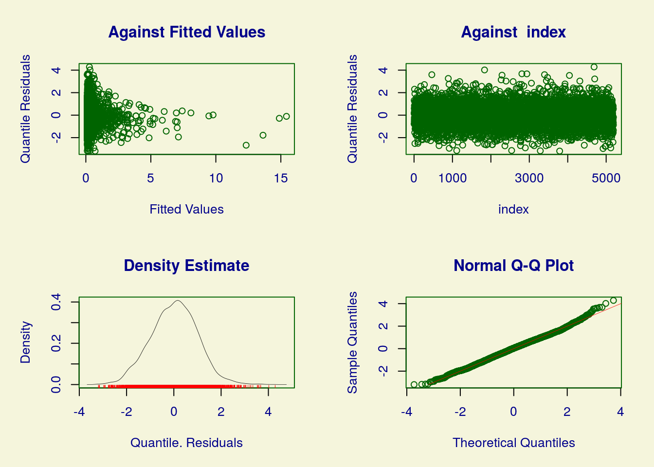

plot(modelo2)

## ******************************************************************
##   Summary of the Randomised Quantile Residuals
##                            mean   =  0.01253109 
##                        variance   =  0.9658382 
##                coef. of skewness  =  0.01900208 
##                coef. of kurtosis  =  3.195999 
## Filliben correlation coefficient  =  0.9991059 
## ******************************************************************

A análise de resíduos indica melhor ajuste em relação ao modelo de Poisson. Mas ainda se observa algum desajuste.

##Modelo 3: Poisson com inflação de zeros

(mas sem covariáveis para o componente do excesso de zeros)

help("ZIP")
modelo3 <- gamlss(doctorco ~ sex + age + agesq + income + levyplus + illness + 
                      actdays + chcond1 + hospadmi + medicine,
                  family = ZIP, data = dvisits) 

## GAMLSS-RS iteration 1: Global Deviance = 6535.095 
## GAMLSS-RS iteration 2: Global Deviance = 6522.272 
## GAMLSS-RS iteration 3: Global Deviance = 6517.939 
## GAMLSS-RS iteration 4: Global Deviance = 6516.39 
## GAMLSS-RS iteration 5: Global Deviance = 6515.82 
## GAMLSS-RS iteration 6: Global Deviance = 6515.607 
## GAMLSS-RS iteration 7: Global Deviance = 6515.527 
## GAMLSS-RS iteration 8: Global Deviance = 6515.495 
## GAMLSS-RS iteration 9: Global Deviance = 6515.482 
## GAMLSS-RS iteration 10: Global Deviance = 6515.477 
## GAMLSS-RS iteration 11: Global Deviance = 6515.475 
## GAMLSS-RS iteration 12: Global Deviance = 6515.474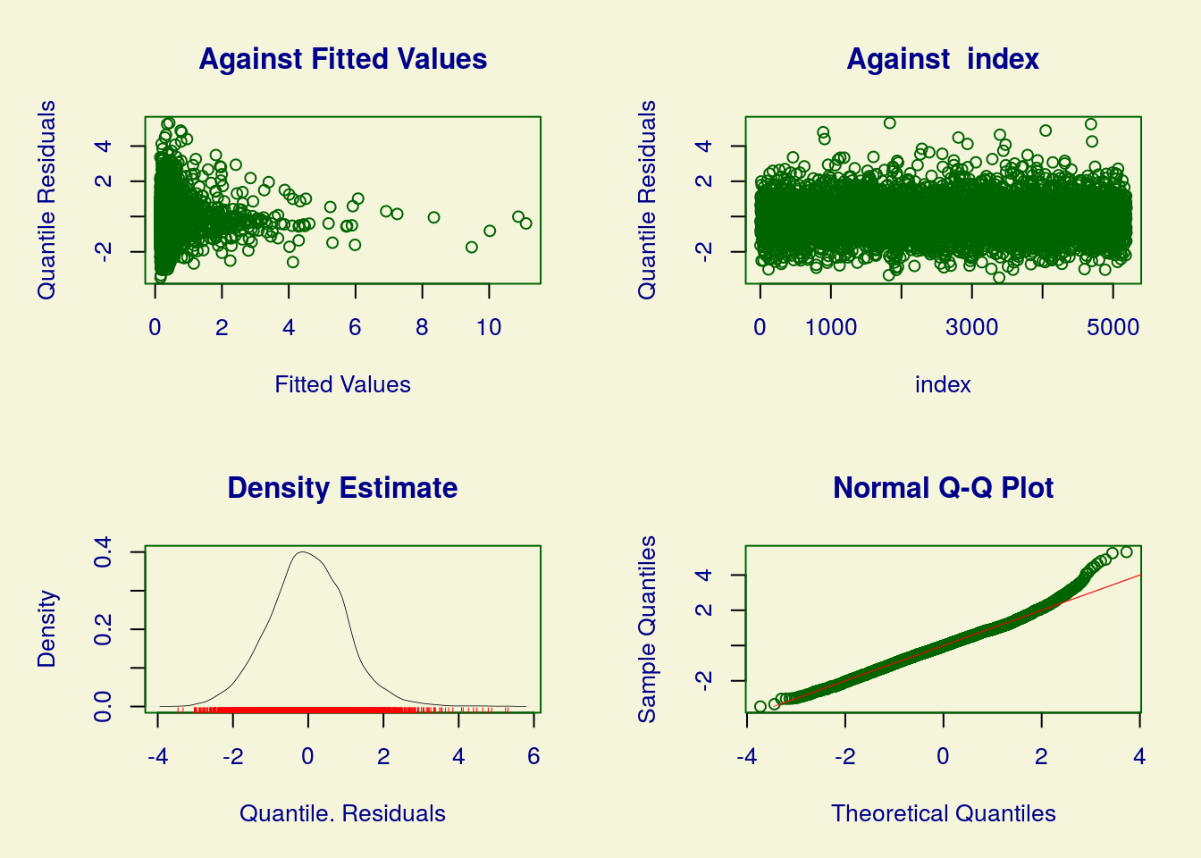

plot(modelo3)

## ******************************************************************
##   Summary of the Randomised Quantile Residuals
##                            mean   =  -0.01944443 
##                        variance   =  1.055439 
##                coef. of skewness  =  0.2321606 
##                coef. of kurtosis  =  3.886979 
## Filliben correlation coefficient  =  0.9963863 
## ******************************************************************

Problemas de ajuste semelhantes ao modelo de Poisson sem inflação.

Modelo 4: Binomial negativa com inflação de zeros

(mas sem covariáveis para o componente do excesso de zeros)

help("ZINBI")
modelo4 <- gamlss(doctorco ~ sex + age + agesq + income + levyplus + illness + 
                      actdays + chcond1 + hospadmi + medicine,
                  family = ZINBI, data = dvisits) 

## GAMLSS-RS iteration 1: Global Deviance = 6434.662 
## GAMLSS-RS iteration 2: Global Deviance = 6394.963 
## GAMLSS-RS iteration 3: Global Deviance = 6379.93 
## GAMLSS-RS iteration 4: Global Deviance = 6370.846 
## GAMLSS-RS iteration 5: Global Deviance = 6365.247 
## GAMLSS-RS iteration 6: Global Deviance = 6361.725 
## GAMLSS-RS iteration 7: Global Deviance = 6359.463 
## GAMLSS-RS iteration 8: Global Deviance = 6357.991 
## GAMLSS-RS iteration 9: Global Deviance = 6357.387 
## GAMLSS-RS iteration 10: Global Deviance = 6357.372 
## GAMLSS-RS iteration 11: Global Deviance = 6357.372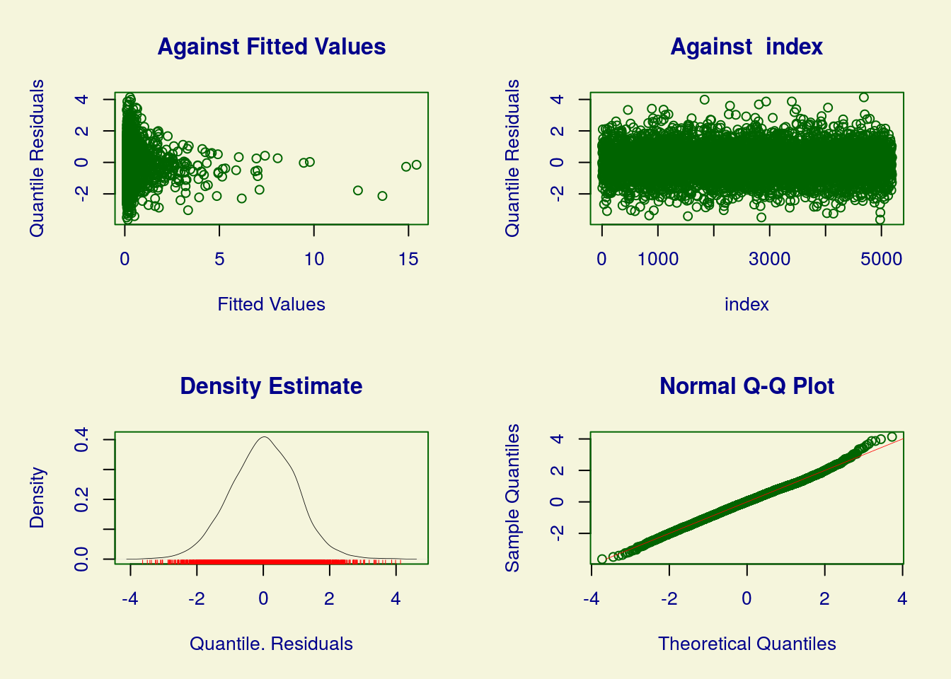

plot(modelo4)

## ******************************************************************
##   Summary of the Randomised Quantile Residuals
##                            mean   =  0.006675355 
##                        variance   =  0.9929617 
##                coef. of skewness  =  -0.00746178 
##                coef. of kurtosis  =  3.306128 
## Filliben correlation coefficient  =  0.9992312 
## ******************************************************************

Modelo 5: Poisson com inflação de zeros

(incluindo as covariáveis também na modelagem do componente do excesso de zeros)

modelo5 <- gamlss(doctorco ~ sex + age + agesq + income + levyplus + illness + 
                      actdays + chcond1 + hospadmi + medicine,
                     sigma.formula = ~ sex + age + agesq + income + levyplus + 
                      illness + actdays + chcond1 + hospadmi + medicine, 
                     family = ZIP, data = dvisits) 

## GAMLSS-RS iteration 1: Global Deviance = 6510.456 
## GAMLSS-RS iteration 2: Global Deviance = 6384.869 
## GAMLSS-RS iteration 3: Global Deviance = 6292.056 
## GAMLSS-RS iteration 4: Global Deviance = 6266.655 
## GAMLSS-RS iteration 5: Global Deviance = 6256.481 
## GAMLSS-RS iteration 6: Global Deviance = 6252.43 
## GAMLSS-RS iteration 7: Global Deviance = 6250.854 
## GAMLSS-RS iteration 8: Global Deviance = 6250.253 
## GAMLSS-RS iteration 9: Global Deviance = 6250.026 
## GAMLSS-RS iteration 10: Global Deviance = 6249.942 
## GAMLSS-RS iteration 11: Global Deviance = 6249.911 
## GAMLSS-RS iteration 12: Global Deviance = 6249.899 
## GAMLSS-RS iteration 13: Global Deviance = 6249.894 
## GAMLSS-RS iteration 14: Global Deviance = 6249.892 
## GAMLSS-RS iteration 15: Global Deviance = 6249.891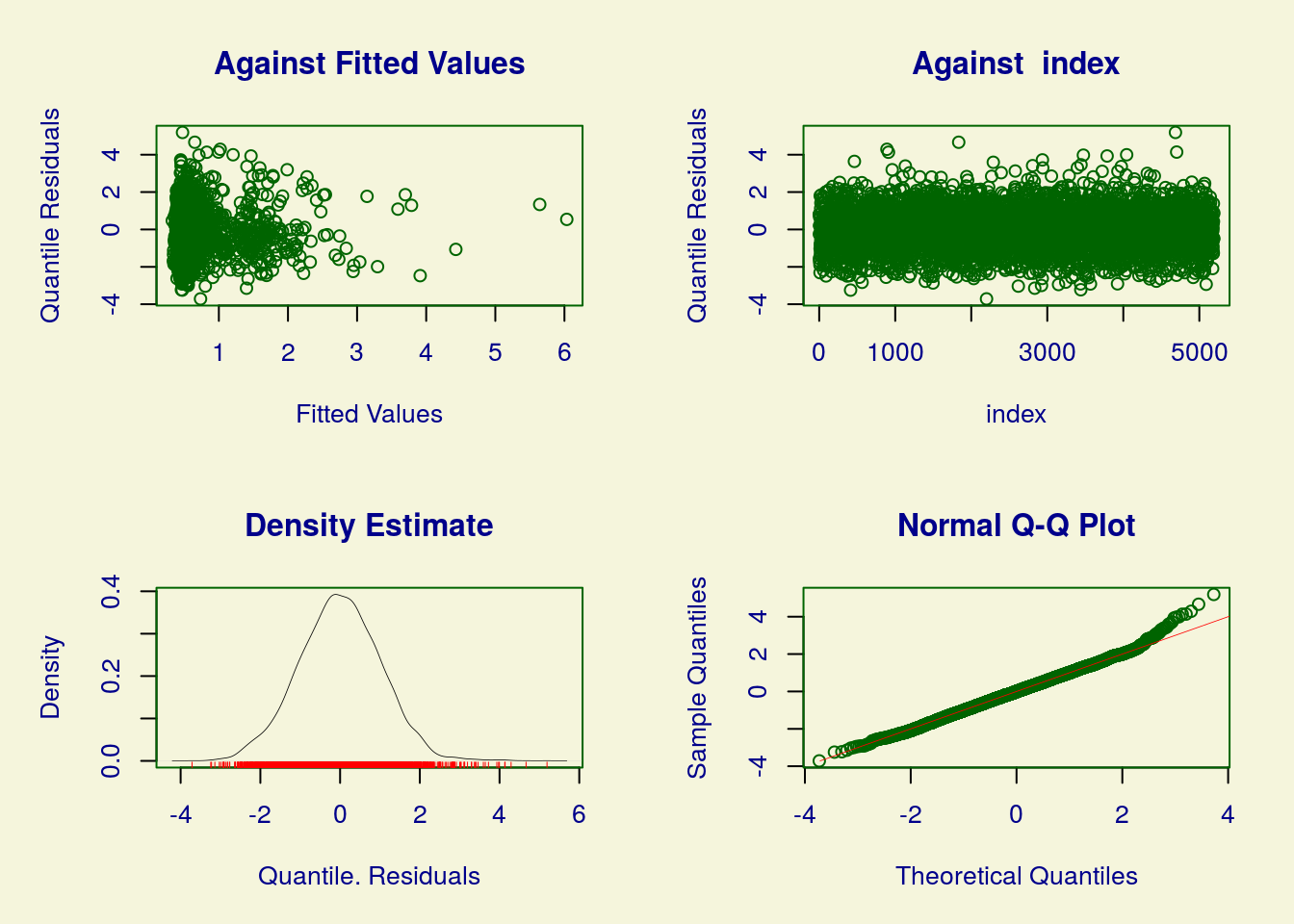

plot(modelo5)

## ******************************************************************
##   Summary of the Randomised Quantile Residuals
##                            mean   =  -0.001643474 
##                        variance   =  1.056911 
##                coef. of skewness  =  0.1074494 
##                coef. of kurtosis  =  3.393902 
## Filliben correlation coefficient  =  0.9986883 
## ******************************************************************

Observe que para incluir covariáveis na modelagem do parâmetro do excesso de zeros, tivemos que declarar uma segunda fórmula em “sigma.formula = ~ …”

Modelo 6: Binomial negativa com inflação de zeros

(incluindo as covariáveis também na modelagem do componente do excesso de zeros)

modelo6 <- gamlss(doctorco ~ sex + age + agesq + income + levyplus + illness + 
                      actdays + chcond1 + hospadmi + medicine,
                  nu.formula = ~ sex + age + agesq + income + levyplus + 
                      illness + actdays + chcond1 + hospadmi + medicine,
                  family = ZINBI, data = dvisits) 

## GAMLSS-RS iteration 1: Global Deviance = 6390.986 
## GAMLSS-RS iteration 2: Global Deviance = 6196.292 
## GAMLSS-RS iteration 3: Global Deviance = 6152.73 
## GAMLSS-RS iteration 4: Global Deviance = 6146.837 
## GAMLSS-RS iteration 5: Global Deviance = 6145.174 
## GAMLSS-RS iteration 6: Global Deviance = 6144.508 
## GAMLSS-RS iteration 7: Global Deviance = 6144.202 
## GAMLSS-RS iteration 8: Global Deviance = 6144.055 
## GAMLSS-RS iteration 9: Global Deviance = 6143.983 
## GAMLSS-RS iteration 10: Global Deviance = 6143.951 
## GAMLSS-RS iteration 11: Global Deviance = 6143.934 
## GAMLSS-RS iteration 12: Global Deviance = 6143.926 
## GAMLSS-RS iteration 13: Global Deviance = 6143.921 
## GAMLSS-RS iteration 14: Global Deviance = 6143.919 
## GAMLSS-RS iteration 15: Global Deviance = 6143.917 
## GAMLSS-RS iteration 16: Global Deviance = 6143.917

plot(modelo6)

## ******************************************************************
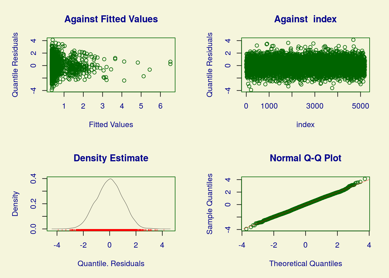
##   Summary of the Randomised Quantile Residuals
##                            mean   =  -0.003352731 
##                        variance   =  1.003999 
##                coef. of skewness  =  -0.04096202 
##                coef. of kurtosis  =  3.083735 
## Filliben correlation coefficient  =  0.9997122 
## ******************************************************************

No caso da binomial negativa, para incluir covariáveis na modelagem do parâmetro do excesso de zeros, tivemos que declarar uma segunda fórmula em “nu.formula = ~ …”. Isso porque, para a ZINB, o gamlss identifica sigma como o parâmetro de dispersão.

Vamos comparar os modelos pelos respectivos AICs.

AIC(modelo1, modelo2, modelo3, modelo4, modelo5, modelo6)

##         df      AIC
## modelo6 23 6189.917
## modelo5 22 6293.891
## modelo2 12 6381.371
## modelo4 13 6383.371
## modelo3 12 6539.474
## modelo1 11 6650.372

Observe que o modelo 6 (ZIBN com covariáveis para o excesso de zeros) foi aquele que produziu menor AIC. Pelos gráficos de resíduos, adicionalmente, fica claro que é o que proporciona melhor ajuste. Vamos explorar um pouco mais ele.

summary(modelo6)

## ******************************************************************
## Family:  c("ZINBI", "Zero inflated negative binomial type I") 
## 
## Call:  gamlss(formula = doctorco ~ sex + age + agesq + income +  
##     levyplus + illness + actdays + chcond1 + hospadmi +  
##     medicine, nu.formula = ~sex + age + agesq + income +  
##     levyplus + illness + actdays + chcond1 + hospadmi +  
##     medicine, family = ZINBI, data = dvisits) 
## 
## Fitting method: RS() 
## 
## ------------------------------------------------------------------
## Mu link function:  log
## Mu Coefficients:
##                     Estimate Std. Error t value Pr(>|t|)    
## (Intercept)        -0.987495   0.282509  -3.495 0.000477 ***
## sexFeminino        -0.031482   0.081265  -0.387 0.698471    
## age                 0.573766   1.451491   0.395 0.692642    
## agesq              -0.890723   1.567536  -0.568 0.569903    
## income             -0.108776   0.126754  -0.858 0.390840    
## levyplusParticular -0.033365   0.079749  -0.418 0.675688    
## illness             0.024569   0.029703   0.827 0.408193    
## actdays             0.089471   0.007236  12.364  < 2e-16 ***
## chcond1Cronico     -0.025228   0.080358  -0.314 0.753575    
## hospadmi            0.201647   0.043833   4.600 4.32e-06 ***
## medicine            0.063351   0.022732   2.787 0.005341 ** 
## ---
## Signif. codes:  0 '***' 0.001 '**' 0.01 '*' 0.05 '.' 0.1 ' ' 1
## 
## ------------------------------------------------------------------
## Sigma link function:  log
## Sigma Coefficients:
##             Estimate Std. Error t value Pr(>|t|)    
## (Intercept)  -0.7149     0.1459  -4.899 9.94e-07 ***
## ---
## Signif. codes:  0 '***' 0.001 '**' 0.01 '*' 0.05 '.' 0.1 ' ' 1
## 
## ------------------------------------------------------------------
## Nu link function:  logit 
## Nu Coefficients:
##                    Estimate Std. Error t value Pr(>|t|)    
## (Intercept)         1.35894    0.71789   1.893  0.05842 .  
## sexFeminino        -0.42549    0.21641  -1.966  0.04934 *  
## age                 5.47141    4.20976   1.300  0.19376    
## agesq              -8.80309    4.81515  -1.828  0.06758 .  
## income             -0.04045    0.33542  -0.121  0.90402    
## levyplusParticular -0.31691    0.22369  -1.417  0.15662    
## illness            -0.57184    0.12925  -4.424 9.87e-06 ***
## actdays            -1.55892    0.52896  -2.947  0.00322 ** 
## chcond1Cronico      0.12111    0.23266   0.521  0.60270    
## hospadmi           -0.35096    0.21280  -1.649  0.09916 .  
## medicine           -0.56346    0.12364  -4.557 5.30e-06 ***
## ---
## Signif. codes:  0 '***' 0.001 '**' 0.01 '*' 0.05 '.' 0.1 ' ' 1
## 
## ------------------------------------------------------------------
## No. of observations in the fit:  5190 
## Degrees of Freedom for the fit:  23
##       Residual Deg. of Freedom:  5167 
##                       at cycle:  16 
##  
## Global Deviance:     6143.917 
##             AIC:     6189.917 
##             SBC:     6340.67 
## ******************************************************************

Observe que o resumo do modelo é separado em duas partes: a primeira para a média da binomial negativa e a segunda para a probabilidade de zeros excedentes.

Podemos observar que a probabilidade associada ao excesso de zeros é menor para pacientes do sexo feminino; diminui conforme o número de enfermidades nas últimas duas semanas (illness); diminui conforme o número de dias inativos nas últimas duas semanas (actdays); diminui conforme o número de medicações prescritas nas últimas duas semanas (medicine).

Ao olhar para a parte da binomial negativa, verificamos que a frequência de consultas, em média, aumenta conforme o número de dias inativos (actdays); aumenta conforme o número de noites internado (hospadmi) e aumenta conforme o número de medicações prescritas (medicine).

Deixo como tarefa escrever as expressões dos modelos ajustados e explorar os efeitos.

Apenas para fins de ilustração, vamos ajustar um modelo apenas com as variáveis com efeito marginalmente significativo ao nível de 5% (além da idade, para o componente do excesso de zeros).

Modelo 7

modelo7 <- gamlss(doctorco ~ actdays + hospadmi + medicine,
                  nu.formula = ~ sex + age + agesq +illness + actdays + medicine,
                  family = ZINBI, data = dvisits)

## GAMLSS-RS iteration 1: Global Deviance = 6306.03 
## GAMLSS-RS iteration 2: Global Deviance = 6163.858 
## GAMLSS-RS iteration 3: Global Deviance = 6158.019 
## GAMLSS-RS iteration 4: Global Deviance = 6155.61 
## GAMLSS-RS iteration 5: Global Deviance = 6154.486 
## GAMLSS-RS iteration 6: Global Deviance = 6153.968 
## GAMLSS-RS iteration 7: Global Deviance = 6153.731 
## GAMLSS-RS iteration 8: Global Deviance = 6153.623 
## GAMLSS-RS iteration 9: Global Deviance = 6153.575 
## GAMLSS-RS iteration 10: Global Deviance = 6153.553 
## GAMLSS-RS iteration 11: Global Deviance = 6153.542 
## GAMLSS-RS iteration 12: Global Deviance = 6153.538 
## GAMLSS-RS iteration 13: Global Deviance = 6153.535 
## GAMLSS-RS iteration 14: Global Deviance = 6153.534 
## GAMLSS-RS iteration 15: Global Deviance = 6153.534

LR.test(modelo7, modelo6) ### Comparando os modelos via teste da razão de verossimilhanças.

##  Likelihood Ratio Test for nested GAMLSS models. 
##  (No check whether the models are nested is performed). 
##  
##        Null model: deviance= 6153.534 with  12 deg. of freedom 
##  Altenative model: deviance= 6143.917 with  23 deg. of freedom 
##  
##  LRT = 9.617128 with 11 deg. of freedom and p-value= 0.5651195

Os ajustes não diferem significativamente. Podemos adotar o modelo 7, portanto.

plot(modelo7)

## ******************************************************************
##   Summary of the Randomised Quantile Residuals
##                            mean   =  -0.0001283558 
##                        variance   =  1.001868 
##                coef. of skewness  =  -0.008838728 
##                coef. of kurtosis  =  2.989365 
## Filliben correlation coefficient  =  0.999719 
## ******************************************************************

summary(modelo7)

## ******************************************************************
## Family:  c("ZINBI", "Zero inflated negative binomial type I") 
## 
## Call:  gamlss(formula = doctorco ~ actdays + hospadmi + medicine,  
##     nu.formula = ~sex + age + agesq + illness + actdays +  
##         medicine, family = ZINBI, data = dvisits) 
## 
## Fitting method: RS() 
## 
## ------------------------------------------------------------------
## Mu link function:  log
## Mu Coefficients:
##              Estimate Std. Error t value Pr(>|t|)    
## (Intercept) -1.009562   0.076839  -13.14  < 2e-16 ***
## actdays      0.089786   0.007152   12.55  < 2e-16 ***
## hospadmi     0.229396   0.041407    5.54 3.17e-08 ***
## medicine     0.060010   0.018755    3.20  0.00138 ** 
## ---
## Signif. codes:  0 '***' 0.001 '**' 0.01 '*' 0.05 '.' 0.1 ' ' 1
## 
## ------------------------------------------------------------------
## Sigma link function:  log
## Sigma Coefficients:
##             Estimate Std. Error t value Pr(>|t|)    
## (Intercept)  -0.7084     0.1432  -4.948 7.75e-07 ***
## ---
## Signif. codes:  0 '***' 0.001 '**' 0.01 '*' 0.05 '.' 0.1 ' ' 1
## 
## ------------------------------------------------------------------
## Nu link function:  logit 
## Nu Coefficients:
##             Estimate Std. Error t value Pr(>|t|)    
## (Intercept)   1.2947     0.5933   2.182  0.02914 *  
## sexFeminino  -0.3999     0.1734  -2.306  0.02114 *  
## age           4.4765     3.1797   1.408  0.15923    
## agesq        -7.1446     3.5822  -1.994  0.04616 *  
## illness      -0.5974     0.1078  -5.540 3.17e-08 ***
## actdays      -1.7479     0.6220  -2.810  0.00497 ** 
## medicine     -0.5831     0.1124  -5.189 2.20e-07 ***
## ---
## Signif. codes:  0 '***' 0.001 '**' 0.01 '*' 0.05 '.' 0.1 ' ' 1
## 
## ------------------------------------------------------------------
## No. of observations in the fit:  5190 
## Degrees of Freedom for the fit:  12
##       Residual Deg. of Freedom:  5178 
##                       at cycle:  15 
##  
## Global Deviance:     6153.534 
##             AIC:     6177.534 
##             SBC:     6256.188 
## ******************************************************************

Embora as estimativas, numericamente, tenham sido alteradas, as conclusões apresentadas anteriormente se mantém.

confint(modelo7, what = 'mu')

##                   2.5 %      97.5 %
## (Intercept) -1.16016348 -0.85896040
## actdays      0.07576936  0.10380296
## hospadmi     0.14823957  0.31055327
## medicine     0.02325016  0.09676993

confint(modelo7, what = 'nu')

##                   2.5 %      97.5 %
## (Intercept)   1.1440569  1.44525995
## sexFeminino  -0.7396899 -0.06004108
## age          -1.7555109 10.70859993
## agesq       -14.1656515 -0.12352664
## illness      -0.8086798 -0.38604047
## actdays      -1.7619162 -1.73388261
## medicine     -0.6198519 -0.54633217

Intervalos de confiança.

pmu <- predict(modelo7, what = 'mu', type = 'response')

Valores ajustados para a média da binomial negativa para cada linha da base.

pnu <- predict(modelo7, what = 'nu', type = 'response')

Valores ajustados para a probabilidade de zero excedente para cada linha da base.

valores <- pmu * (1-pnu)
head(valores)

##       2096       2434       4314        931       4698       1968 
## 0.22980636 0.38092510 0.04793570 0.32713137 0.11978515 0.08701931

Valores ajustados para o número esperado de consultas para cada linha da base.