Regressão para dados binários - modelo preditivo

require(kernlab)
require(statmod)
require(pROC)
require(car)
require(glmnet)

Vamos usar regressão logística para classificar e-mails como spams ou não spams segundo as frequências com que diferentes termos e caracteres aparecem no corpo da mensagem.

data("spam")
help("spam")
summary(spam)

##       make           address            all             num3d         
##  Min.   :0.0000   Min.   : 0.000   Min.   :0.0000   Min.   : 0.00000  
##  1st Qu.:0.0000   1st Qu.: 0.000   1st Qu.:0.0000   1st Qu.: 0.00000  
##  Median :0.0000   Median : 0.000   Median :0.0000   Median : 0.00000  
##  Mean   :0.1046   Mean   : 0.213   Mean   :0.2807   Mean   : 0.06542  
##  3rd Qu.:0.0000   3rd Qu.: 0.000   3rd Qu.:0.4200   3rd Qu.: 0.00000  
##  Max.   :4.5400   Max.   :14.280   Max.   :5.1000   Max.   :42.81000  
##       our               over            remove          internet      
##  Min.   : 0.0000   Min.   :0.0000   Min.   :0.0000   Min.   : 0.0000  
##  1st Qu.: 0.0000   1st Qu.:0.0000   1st Qu.:0.0000   1st Qu.: 0.0000  
##  Median : 0.0000   Median :0.0000   Median :0.0000   Median : 0.0000  
##  Mean   : 0.3122   Mean   :0.0959   Mean   :0.1142   Mean   : 0.1053  
##  3rd Qu.: 0.3800   3rd Qu.:0.0000   3rd Qu.:0.0000   3rd Qu.: 0.0000  
##  Max.   :10.0000   Max.   :5.8800   Max.   :7.2700   Max.   :11.1100  
##      order              mail            receive             will       
##  Min.   :0.00000   Min.   : 0.0000   Min.   :0.00000   Min.   :0.0000  
##  1st Qu.:0.00000   1st Qu.: 0.0000   1st Qu.:0.00000   1st Qu.:0.0000  
##  Median :0.00000   Median : 0.0000   Median :0.00000   Median :0.1000  
##  Mean   :0.09007   Mean   : 0.2394   Mean   :0.05982   Mean   :0.5417  
##  3rd Qu.:0.00000   3rd Qu.: 0.1600   3rd Qu.:0.00000   3rd Qu.:0.8000  
##  Max.   :5.26000   Max.   :18.1800   Max.   :2.61000   Max.   :9.6700  
##      people            report           addresses           free        
##  Min.   :0.00000   Min.   : 0.00000   Min.   :0.0000   Min.   : 0.0000  
##  1st Qu.:0.00000   1st Qu.: 0.00000   1st Qu.:0.0000   1st Qu.: 0.0000  
##  Median :0.00000   Median : 0.00000   Median :0.0000   Median : 0.0000  
##  Mean   :0.09393   Mean   : 0.05863   Mean   :0.0492   Mean   : 0.2488  
##  3rd Qu.:0.00000   3rd Qu.: 0.00000   3rd Qu.:0.0000   3rd Qu.: 0.1000  
##  Max.   :5.55000   Max.   :10.00000   Max.   :4.4100   Max.   :20.0000  
##     business          email             you             credit        
##  Min.   :0.0000   Min.   :0.0000   Min.   : 0.000   Min.   : 0.00000  
##  1st Qu.:0.0000   1st Qu.:0.0000   1st Qu.: 0.000   1st Qu.: 0.00000  
##  Median :0.0000   Median :0.0000   Median : 1.310   Median : 0.00000  
##  Mean   :0.1426   Mean   :0.1847   Mean   : 1.662   Mean   : 0.08558  
##  3rd Qu.:0.0000   3rd Qu.:0.0000   3rd Qu.: 2.640   3rd Qu.: 0.00000  
##  Max.   :7.1400   Max.   :9.0900   Max.   :18.750   Max.   :18.18000  
##       your              font             num000           money         
##  Min.   : 0.0000   Min.   : 0.0000   Min.   :0.0000   Min.   : 0.00000  
##  1st Qu.: 0.0000   1st Qu.: 0.0000   1st Qu.:0.0000   1st Qu.: 0.00000  
##  Median : 0.2200   Median : 0.0000   Median :0.0000   Median : 0.00000  
##  Mean   : 0.8098   Mean   : 0.1212   Mean   :0.1016   Mean   : 0.09427  
##  3rd Qu.: 1.2700   3rd Qu.: 0.0000   3rd Qu.:0.0000   3rd Qu.: 0.00000  
##  Max.   :11.1100   Max.   :17.1000   Max.   :5.4500   Max.   :12.50000  
##        hp               hpl              george            num650      
##  Min.   : 0.0000   Min.   : 0.0000   Min.   : 0.0000   Min.   :0.0000  
##  1st Qu.: 0.0000   1st Qu.: 0.0000   1st Qu.: 0.0000   1st Qu.:0.0000  
##  Median : 0.0000   Median : 0.0000   Median : 0.0000   Median :0.0000  
##  Mean   : 0.5495   Mean   : 0.2654   Mean   : 0.7673   Mean   :0.1248  
##  3rd Qu.: 0.0000   3rd Qu.: 0.0000   3rd Qu.: 0.0000   3rd Qu.:0.0000  
##  Max.   :20.8300   Max.   :16.6600   Max.   :33.3300   Max.   :9.0900  
##       lab                labs            telnet             num857       
##  Min.   : 0.00000   Min.   :0.0000   Min.   : 0.00000   Min.   :0.00000  
##  1st Qu.: 0.00000   1st Qu.:0.0000   1st Qu.: 0.00000   1st Qu.:0.00000  
##  Median : 0.00000   Median :0.0000   Median : 0.00000   Median :0.00000  
##  Mean   : 0.09892   Mean   :0.1029   Mean   : 0.06475   Mean   :0.04705  
##  3rd Qu.: 0.00000   3rd Qu.:0.0000   3rd Qu.: 0.00000   3rd Qu.:0.00000  
##  Max.   :14.28000   Max.   :5.8800   Max.   :12.50000   Max.   :4.76000  
##       data              num415            num85           technology     
##  Min.   : 0.00000   Min.   :0.00000   Min.   : 0.0000   Min.   :0.00000  
##  1st Qu.: 0.00000   1st Qu.:0.00000   1st Qu.: 0.0000   1st Qu.:0.00000  
##  Median : 0.00000   Median :0.00000   Median : 0.0000   Median :0.00000  
##  Mean   : 0.09723   Mean   :0.04784   Mean   : 0.1054   Mean   :0.09748  
##  3rd Qu.: 0.00000   3rd Qu.:0.00000   3rd Qu.: 0.0000   3rd Qu.:0.00000  
##  Max.   :18.18000   Max.   :4.76000   Max.   :20.0000   Max.   :7.69000  
##     num1999          parts              pm               direct       
##  Min.   :0.000   Min.   :0.0000   Min.   : 0.00000   Min.   :0.00000  
##  1st Qu.:0.000   1st Qu.:0.0000   1st Qu.: 0.00000   1st Qu.:0.00000  
##  Median :0.000   Median :0.0000   Median : 0.00000   Median :0.00000  
##  Mean   :0.137   Mean   :0.0132   Mean   : 0.07863   Mean   :0.06483  
##  3rd Qu.:0.000   3rd Qu.:0.0000   3rd Qu.: 0.00000   3rd Qu.:0.00000  
##  Max.   :6.890   Max.   :8.3300   Max.   :11.11000   Max.   :4.76000  
##        cs             meeting           original         project       
##  Min.   :0.00000   Min.   : 0.0000   Min.   :0.0000   Min.   : 0.0000  
##  1st Qu.:0.00000   1st Qu.: 0.0000   1st Qu.:0.0000   1st Qu.: 0.0000  
##  Median :0.00000   Median : 0.0000   Median :0.0000   Median : 0.0000  
##  Mean   :0.04367   Mean   : 0.1323   Mean   :0.0461   Mean   : 0.0792  
##  3rd Qu.:0.00000   3rd Qu.: 0.0000   3rd Qu.:0.0000   3rd Qu.: 0.0000  
##  Max.   :7.14000   Max.   :14.2800   Max.   :3.5700   Max.   :20.0000  
##        re               edu              table            conference      
##  Min.   : 0.0000   Min.   : 0.0000   Min.   :0.000000   Min.   : 0.00000  
##  1st Qu.: 0.0000   1st Qu.: 0.0000   1st Qu.:0.000000   1st Qu.: 0.00000  
##  Median : 0.0000   Median : 0.0000   Median :0.000000   Median : 0.00000  
##  Mean   : 0.3012   Mean   : 0.1798   Mean   :0.005444   Mean   : 0.03187  
##  3rd Qu.: 0.1100   3rd Qu.: 0.0000   3rd Qu.:0.000000   3rd Qu.: 0.00000  
##  Max.   :21.4200   Max.   :22.0500   Max.   :2.170000   Max.   :10.00000  
##  charSemicolon     charRoundbracket charSquarebracket charExclamation  
##  Min.   :0.00000   Min.   :0.000    Min.   :0.00000   Min.   : 0.0000  
##  1st Qu.:0.00000   1st Qu.:0.000    1st Qu.:0.00000   1st Qu.: 0.0000  
##  Median :0.00000   Median :0.065    Median :0.00000   Median : 0.0000  
##  Mean   :0.03857   Mean   :0.139    Mean   :0.01698   Mean   : 0.2691  
##  3rd Qu.:0.00000   3rd Qu.:0.188    3rd Qu.:0.00000   3rd Qu.: 0.3150  
##  Max.   :4.38500   Max.   :9.752    Max.   :4.08100   Max.   :32.4780  
##    charDollar         charHash          capitalAve        capitalLong     
##  Min.   :0.00000   Min.   : 0.00000   Min.   :   1.000   Min.   :   1.00  
##  1st Qu.:0.00000   1st Qu.: 0.00000   1st Qu.:   1.588   1st Qu.:   6.00  
##  Median :0.00000   Median : 0.00000   Median :   2.276   Median :  15.00  
##  Mean   :0.07581   Mean   : 0.04424   Mean   :   5.191   Mean   :  52.17  
##  3rd Qu.:0.05200   3rd Qu.: 0.00000   3rd Qu.:   3.706   3rd Qu.:  43.00  
##  Max.   :6.00300   Max.   :19.82900   Max.   :1102.500   Max.   :9989.00  
##   capitalTotal          type     
##  Min.   :    1.0   nonspam:2788  
##  1st Qu.:   35.0   spam   :1813  
##  Median :   95.0                 
##  Mean   :  283.3                 
##  3rd Qu.:  266.0                 
##  Max.   :15841.0

Vamos selecionar apenas as covariáveis com frequência média superior a 0.2 para a sequência da análise.

i_freq <- which(apply(spam[,1:57],2,mean) > 0.2)
spam2 <- spam[,c(i_freq, 58)]

Alguns gráficos

with(spam2, boxplot(log(charExclamation + 0.1) ~ type, ylab = 'log(frequência)',
                   col = 'lightblue', cex = 1.45, las = 1))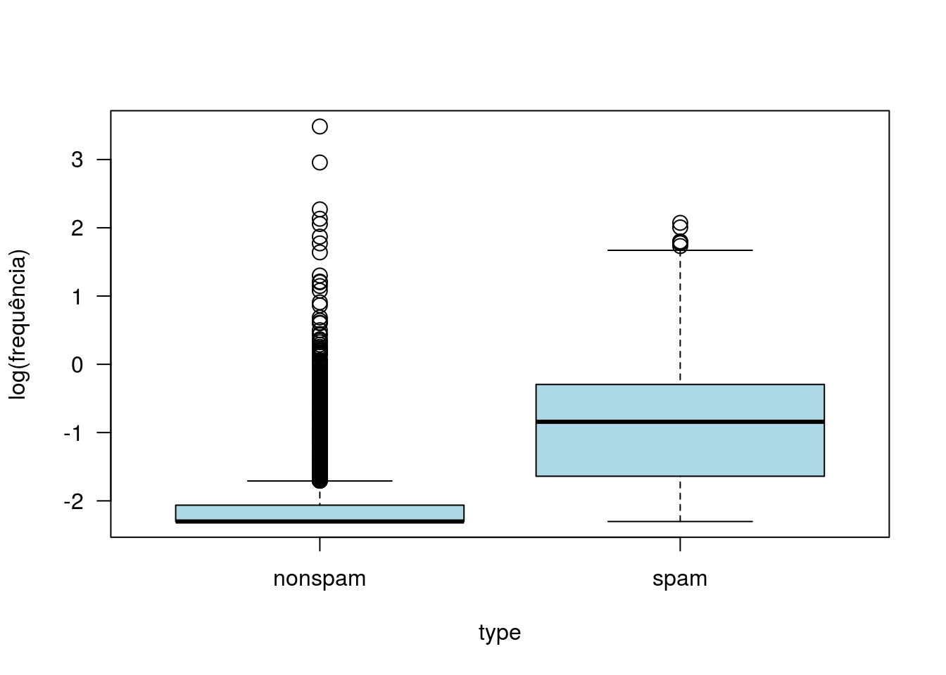

with(spam2, boxplot(log(capitalTotal + 0.1) ~ type, ylab = 'log(frequência)',
                   col = 'lightblue', cex = 1.45, las = 1))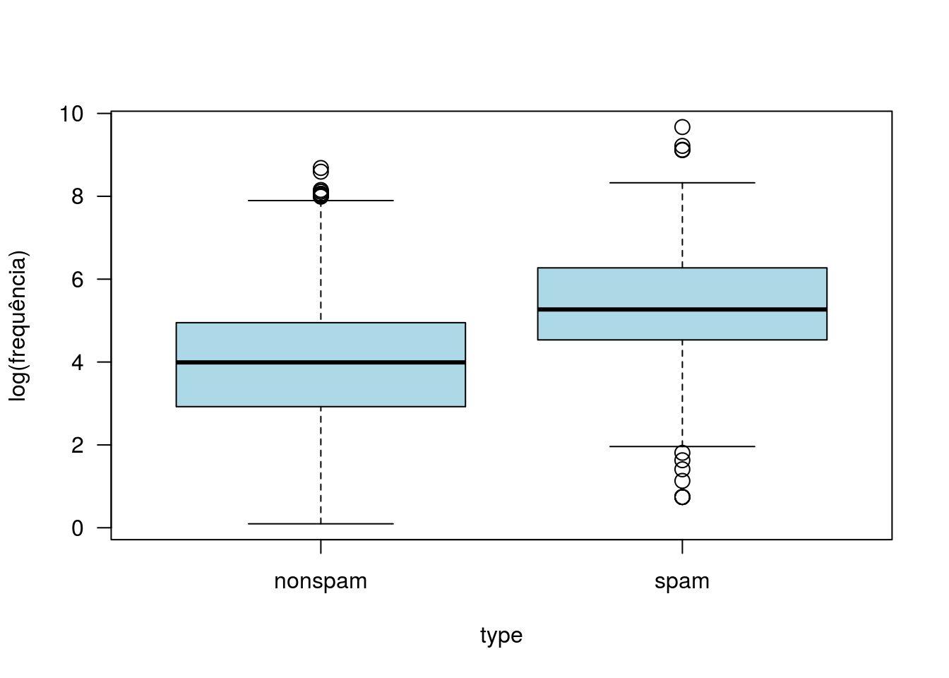

Aparentemente, as frequências de pontos de exclamação ou letras maiúsculas são importantes para discriminar spams e não spams (spams têm maior frequência de ambos).

Preparação dos dados

Vamos dividir a base em duas: uma para ajuste do modelo e outra para validação. A base de validação com 1000 observações e a de ajuste com as demais.

set.seed(88) # Fixando a semente para sorteio das observações.
select <- sample(1:nrow(spam2), 1000)

Linhas da base que serão usadas para validação.

spam_ajuste <- spam2[-select,] # Base de ajuste.
spam_predict <- spam2[select,] # Base de validação.

Ajuste do modelo

Vamos considerar diferentes abordagens:

Modelo 1 - GLM com todas as covariáveis;

modelo1 <- glm(type ~ ., family = 'binomial', data = spam_ajuste)

## Warning: glm.fit: fitted probabilities numerically 0 or 1 occurred

pred1 <- predict(modelo1, newdata = spam_predict, type = 'response')
head(round(pred1,5), n = 10) # Predições.

##    2327    2129     669    3417    3229    3471    3669    1353     839 
## 0.22983 0.01088 0.92569 0.00000 0.00000 0.00004 0.00000 0.78723 0.78501 
##    2645 
## 0.37904

Tabela de confusão e medidas de performance preditiva

class1 <- ifelse(pred1 > 0.5, 'Class_spam', 'Class_nspam')
tabcruz <- table(class1, spam_predict$type)
tabcruz

##              
## class1        nonspam spam
##   Class_nspam     556   66
##   Class_spam       60  318

ac1 <- sum(diag(tabcruz))/1000; ac1 # Acurácia.

## [1] 0.874

s1 <- tabcruz[2,2]/(tabcruz[1,2] + tabcruz[2,2]); s1 # Sensibilidade.

## [1] 0.828125

e1 <- tabcruz[1,1]/(tabcruz[1,1] + tabcruz[2,1]); e1 # Especificidade.

## [1] 0.9025974

Modelo 2

Com seleção do tipo Backward, via AIC

modelo2 <- step(modelo1, k = 2)

## Start:  AIC=2354.97
## type ~ address + all + our + mail + will + free + you + your + 
##     hp + hpl + george + re + charExclamation + capitalAve + capitalLong + 
##     capitalTotal
## 
##                   Df Deviance   AIC
## - all              1     2321  2353
## <none>                   2321  2355
## - address          1     2326  2358
## - capitalAve       1     2327  2359
## - will             1     2333  2365
## - hpl              1     2335  2367
## - capitalTotal     1     2343  2375
## - charExclamation  1     2373  2405
## - your             1     2415  2447
## - free             1     2446  2478
## - george           1     2642  2674
## - capitalLong      1    67402 67434
## - re               1    69132 69164
## - hp               1    73313 73345
## - our              1    73745 73777
## - you              1    73817 73849
## - mail             1    77494 77526
## 
## Step:  AIC=2353.19
## type ~ address + our + mail + will + free + you + your + hp + 
##     hpl + george + re + charExclamation + capitalAve + capitalLong + 
##     capitalTotal
## 
##                   Df Deviance   AIC
## <none>                   2321  2353
## - address          1     2326  2356
## - capitalAve       1     2327  2357
## - will             1     2333  2363
## - capitalTotal     1     2343  2373
## - charExclamation  1     2373  2403
## - our              1     2384  2414
## - your             1     2418  2448
## - free             1     2447  2477
## - george           1     2645  2675
## - hp               1    37341 37371
## - capitalLong      1    45055 45085
## - hpl              1    56228 56258
## - re               1    56589 56619
## - you              1    61779 61809
## - mail             1    78143 78173

pred2 <- predict(modelo2, newdata = spam_predict, type = 'response')

Tabela de confusão e medidas de performance preditiva

class2 <- ifelse(pred2 > 0.5, 'Class_spam', 'Class_nspam')
tabcruz <- table(class2, spam_predict$type)
tabcruz

##              
## class2        nonspam spam
##   Class_nspam     556   65
##   Class_spam       60  319

ac2 <- sum(diag(tabcruz))/1000; ac2 # Acurácia.

## [1] 0.875

s2 <- tabcruz[2,2]/(tabcruz[1,2] + tabcruz[2,2]); s2 # Sensibilidade.

## [1] 0.8307292

e2 <- tabcruz[1,1]/(tabcruz[1,1] + tabcruz[2,1]); e2 # Especificidade.

## [1] 0.9025974

Modelo 3 - com seleção do tipo Backward, via BIC

modelo3 <- step(modelo1, k = log(nrow(spam_ajuste)))

## Start:  AIC=2460.19
## type ~ address + all + our + mail + will + free + you + your + 
##     hp + hpl + george + re + charExclamation + capitalAve + capitalLong + 
##     capitalTotal
## 
##                   Df Deviance   AIC
## - all              1     2321  2452
## - address          1     2326  2457
## - capitalAve       1     2327  2458
## <none>                   2321  2460
## - will             1     2333  2464
## - hpl              1     2335  2467
## - capitalTotal     1     2343  2474
## - charExclamation  1     2373  2504
## - your             1     2415  2546
## - free             1     2446  2577
## - george           1     2642  2773
## - capitalLong      1    67402 67533
## - re               1    69132 69263
## - hp               1    73313 73444
## - our              1    73745 73876
## - you              1    73817 73948
## - mail             1    77494 77625
## 
## Step:  AIC=2452.21
## type ~ address + our + mail + will + free + you + your + hp + 
##     hpl + george + re + charExclamation + capitalAve + capitalLong + 
##     capitalTotal
## 
##                   Df Deviance   AIC
## - address          1     2326  2449
## - capitalAve       1     2327  2450
## <none>                   2321  2452
## - will             1     2333  2455
## - capitalTotal     1     2343  2466
## - charExclamation  1     2373  2496
## - our              1     2384  2506
## - your             1     2418  2541
## - free             1     2447  2570
## - george           1     2645  2768
## - hp               1    37341 37464
## - capitalLong      1    45055 45177
## - hpl              1    56228 56351
## - re               1    56589 56711
## - you              1    61779 61902
## - mail             1    78143 78265
## 
## Step:  AIC=2448.94
## type ~ our + mail + will + free + you + your + hp + hpl + george + 
##     re + charExclamation + capitalAve + capitalLong + capitalTotal
## 
##                   Df Deviance   AIC
## - capitalAve       1     2332  2447
## <none>                   2326  2449
## - will             1     2337  2452
## - capitalTotal     1     2348  2463
## - charExclamation  1     2379  2494
## - our              1     2389  2504
## - your             1     2424  2539
## - free             1     2453  2567
## - george           1     2649  2764
## - you              1    34458 34572
## - hp               1    38495 38609
## - hpl              1    61346 61461
## - capitalLong      1    74322 74437
## - mail             1    78575 78690
## - re               1    86455 86569
## 
## Step:  AIC=2446.54
## type ~ our + mail + will + free + you + your + hp + hpl + george + 
##     re + charExclamation + capitalLong + capitalTotal
## 
##                   Df Deviance    AIC
## - mail             1     2338   2444
## <none>                   2332   2447
## - capitalTotal     1     2351   2458
## - you              1     2356   2463
## - charExclamation  1     2389   2495
## - our              1     2394   2501
## - hp               1     2445   2552
## - capitalLong      1     2457   2563
## - george           1     2649   2756
## - hpl              1    61563  61669
## - your             1    64230  64336
## - will             1    64590  64697
## - free             1    84414  84521
## - re               1   109249 109356
## 
## Step:  AIC=2444.44
## type ~ our + will + free + you + your + hp + hpl + george + re + 
##     charExclamation + capitalLong + capitalTotal
## 
##                   Df Deviance   AIC
## <none>                   2338  2444
## - capitalTotal     1     2357  2455
## - you              1     2364  2463
## - charExclamation  1     2394  2492
## - our              1     2406  2504
## - re               1     2417  2515
## - your             1     2437  2535
## - free             1     2467  2565
## - capitalLong      1     2469  2567
## - george           1     2658  2756
## - hp               1    38927 39025
## - will             1    74322 74420
## - hpl              1    83549 83647

pred3 <- predict(modelo3, newdata = spam_predict, type = 'response')

Tabela de confusão e medidas de performance preditiva

class3 <- ifelse(pred3 > 0.5, 'Class_spam', 'Class_nspam')
tabcruz <- table(class3, spam_predict$type)
tabcruz

##              
## class3        nonspam spam
##   Class_nspam     556   67
##   Class_spam       60  317

ac3 <- sum(diag(tabcruz))/1000; ac3 # Acurácia.

## [1] 0.873

s3 <- tabcruz[2,2]/(tabcruz[1,2] + tabcruz[2,2]); s3 # Sensibilidade.

## [1] 0.8255208

e3 <- tabcruz[1,1]/(tabcruz[1,1] + tabcruz[2,1]); e3 # Especificidade.

## [1] 0.9025974

Modelo 4

Com regularização, método lasso

x <- model.matrix(type ~ ., data = spam_ajuste)[, -1]
y <- ifelse(spam_ajuste$type == 'spam', 1, 0)

modelo4 <- glmnet(x, y, family = 'binomial', alpha = 1)
cvfit <- cv.glmnet(x, y, family = 'binomial', alpha = 1, nfolds = 10)

newx <- model.matrix(type ~ ., data = spam_predict)[, -1]
pred4 <- predict(modelo4, newx = newx, s = cvfit$lambda.min, type = 'response')

Tabela de confusão e medidas de performance preditiva

class4 <- ifelse(pred4 > 0.5, 'Class_spam', 'Class_nspam')
tabcruz <- table(class4, spam_predict$type)
tabcruz

##              
## class4        nonspam spam
##   Class_nspam     554   65
##   Class_spam       62  319

ac4 <- sum(diag(tabcruz))/1000; ac4 # Acurácia.

## [1] 0.873

s4 <- tabcruz[2,2]/(tabcruz[1,2] + tabcruz[2,2]); s4 # Sensibilidade.

## [1] 0.8307292

e4 <- tabcruz[1,1]/(tabcruz[1,1] + tabcruz[2,1]); e4 # Especificidade.

## [1] 0.8993506

Modelo 5

Com regularização, método ridge

x <- model.matrix(type ~ ., data = spam_ajuste)[, -1]
y <- ifelse(spam_ajuste$type == 'spam', 1, 0)

modelo5 <- glmnet(x, y, family = 'binomial', alpha = 0)
cvfit <- cv.glmnet(x, y, family = 'binomial', alpha = 0, nfolds = 10)

newx <- model.matrix(type ~ ., data = spam_predict)[, -1]
pred5 <- predict(modelo5, newx = newx, s = cvfit$lambda.min, type = 'response')

Tabela de confusão e medidas de performance preditiva

class5 <- ifelse(pred5 > 0.5, 'Class_spam', 'Class_nspam')
tabcruz <- table(class5, spam_predict$type)
tabcruz

##              
## class5        nonspam spam
##   Class_nspam     554   88
##   Class_spam       62  296

ac5 <- sum(diag(tabcruz))/1000; ac5 # Acurácia.

## [1] 0.85

s5 <- tabcruz[2,2]/(tabcruz[1,2] + tabcruz[2,2]); s5 # Sensibilidade.

## [1] 0.7708333

e5 <- tabcruz[1,1]/(tabcruz[1,1] + tabcruz[2,1]); e5 # Especificidade.

## [1] 0.8993506

Vários resultados

data.frame(Modelo = c('Modelo 1', 'Modelo 2', 'Modelo 3', 'Modelo 4', 'modelo 5'),
           Acurácia  = c(ac1, ac2, ac3, ac4, ac5), Sensibilidade = c(s1, s2, s3, s4, s5),
           Especificidade = c(e1, e2, e3, e4, e5))

##     Modelo Acurácia Sensibilidade Especificidade
## 1 Modelo 1    0.874     0.8281250      0.9025974
## 2 Modelo 2    0.875     0.8307292      0.9025974
## 3 Modelo 3    0.873     0.8255208      0.9025974
## 4 Modelo 4    0.873     0.8307292      0.8993506
## 5 modelo 5    0.850     0.7708333      0.8993506

Análise via curva ROC

Procurando as regras de classificação (pontos de corte) ótimos.

predroc1 <- roc(spam_predict$type, pred1, percent = TRUE)

## Setting levels: control = nonspam, case = spam

## Setting direction: controls < cases

predroc1$auc

## Area under the curve: 93.8%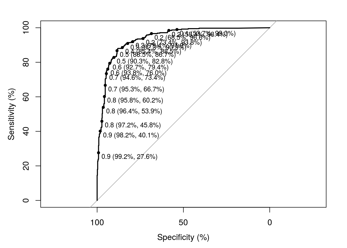

plot(predroc1, print.thres = seq(0.1,0.95,0.05), print.thres.pattern.cex = 0.8)

c1 <- coords(predroc1, 'best'); c1

##   threshold specificity sensitivity 
##   0.4306366  87.9870130  88.0208333

predroc2 <- roc(spam_predict$type, pred2, percent = TRUE)

## Setting levels: control = nonspam, case = spam
## Setting direction: controls < cases

predroc2$auc

## Area under the curve: 93.79%

c2 <- coords(predroc2, 'best'); c2

##   threshold specificity sensitivity 
##   0.4387975  88.1493506  87.7604167

predroc3 <- roc(spam_predict$type, pred3, percent = TRUE)

## Setting levels: control = nonspam, case = spam
## Setting direction: controls < cases

predroc3$auc

## Area under the curve: 93.67%

c3 <- coords(predroc3, 'best'); c3

##   threshold specificity sensitivity 
##   0.4127096  87.0129870  87.5000000

predroc4 <- roc(spam_predict$type, as.numeric(pred4), percent = TRUE)

## Setting levels: control = nonspam, case = spam
## Setting direction: controls < cases

predroc4$auc

## Area under the curve: 93.61%

c4 <- coords(predroc4, 'best'); c4

##   threshold specificity sensitivity 
##   0.4214727  87.1753247  87.5000000

predroc5 <- roc(spam_predict$type, as.numeric(pred5), percent = TRUE)

## Setting levels: control = nonspam, case = spam
## Setting direction: controls < cases

predroc5$auc

## Area under the curve: 91.67%

c5 <- coords(predroc5, 'best'); c5

##   threshold specificity sensitivity 
##   0.4217696  85.5519481  84.6354167

data.frame(Modelo = c('Modelo 1', 'Modelo 2', 'Modelo 3', 'Modelo 4', 'modelo 5'),
           rbind(c1, c2, c3, c4, c5))

##      Modelo threshold specificity sensitivity
## c1 Modelo 1 0.4306366    87.98701    88.02083
## c2 Modelo 2 0.4387975    88.14935    87.76042
## c3 Modelo 3 0.4127096    87.01299    87.50000
## c4 Modelo 4 0.4214727    87.17532    87.50000
## c5 modelo 5 0.4217696    85.55195    84.63542

Incorporando custos de má-classificação

Custos de má-classificação podem ser incorporados na seleção da melhor regra de classificação. A função coords, por default, identifica o ponto de corte tal que a soma sensibilidade + especificidade seja máxima. Podemos modificar este critério através da função best werights, em que declaramos:

1 - O custo relativo de um falso negativo quando comparado a um falso positivo;

2 - A prevalência ou proporção de casos (spams) na população.

Vamos considerar alguns cenários. Em todos os casos, Cn|s é o custo de classificar um spam como não spam, Cs|n o de classificar como spam um não spam e Ps é a prevalência de spams.

# Cenário 1 - Cn|s = 0.5*Cs|n, Ps = 1/3.
coords(predroc1, x = 'best', best.weights = c(0.5, 1/3))

##   threshold specificity sensitivity 
##   0.6343966  94.6428571  75.0000000

# Cenário 2 - Cn|s = Cs|n, Ps = 1/3.
coords(predroc1, x = 'best', best.weights = c(1, 1/3))

##   threshold specificity sensitivity 
##   0.5668292  93.1818182  78.9062500

# Cenário 3 - Cn|s = Cs|n, Ps = 1/2.
coords(predroc1, x = 'best', best.weights = c(1, 1/2))

##   threshold specificity sensitivity 
##   0.4306366  87.9870130  88.0208333

# Cenário 4 - Cn|s = Cs|n, Ps = 1/20.
coords(predroc1, x = 'best', best.weights = c(1, 1/20))

##   threshold specificity sensitivity 
##   0.9200617  99.0259740  36.7187500

# Cenário 5 - Cn|s = 2*Cs|n, Ps = 1/3.
coords(predroc1, x = 'best', best.weights = c(2, 1/3))

##   threshold specificity sensitivity 
##   0.4306366  87.9870130  88.0208333

# Cenário 6 - Cn|s = 5*Cs|n, Ps = 1/3.
coords(predroc1, x = 'best', best.weights = c(5, 1/3))

##   threshold specificity sensitivity 
##   0.2287856  71.2662338  95.8333333

# Cenário 7 - Cn|s = 10*Cs|n, Ps = 1/3.
coords(predroc1, x = 'best', best.weights = c(10, 1/3))

##   threshold specificity sensitivity 
##   0.2030385  68.8311688  96.6145833

Base de dados sobre spams

Cesar Taconeli

Regressão para dados binários - modelo preditivo

Preparação dos dados

Ajuste do modelo

Modelo 2

Modelo 3 - com seleção do tipo Backward, via BIC

Modelo 4

Modelo 5

Vários resultados

Análise via curva ROC

Incorporando custos de má-classificação